

At Doma, we use natural language processing (NLP) as part of our mission to bring faster and more seamless mortgage closings to the U.S.. NLP is the use of mathematics to enable computers to learn and understand human language. Most people have seen this in action when their phone or email client makes a suggestion for the next word or phrase to type. Our NLP toolkit includes Google’s recent groundbreaking advancement in the field – a deep neural network architecture known as the Bidirectional Encoder Representations from Transformers (BERT).
What makes BERT such an appealing technique is its flexibility. At its core, a BERT model learns a deep representation of natural language through its design and being trained on billions of words. This representation can be tweaked and modified with additional data to accomplish a variety of tasks, including question answering, text classification, word replacement, and much more.
The downside of BERT is that, like many deep learning models, it can be difficult to understand the nuances of its behavior and learned representations. We are excited to share some approaches we’ve taken to explore the inner workings of a fine-tuned BERT model.
Visualizing embedding vectors
Completing real estate transactions involves dozens of parties collaborating together, with the majority of the communication between those parties taking place via email. We adapted BERT to solve problems using our email corpus, and wanted to gain a better understanding of how our models created semantic representations of our text data.
In practice, this semantic representation is a vector with 768 dimensions. To understand the subtle differences being learned by the model, we decided to visualize sets of sentences that are similar in meaning and somewhat common in our corpus. For example, we see many variations of people responding affirmatively to a question:
[“It’s correct.”, “It’s ok.”]
Or identifying the presence of a mistake:
[“I made the mistake.”, “This was my mistake.”],
You can find the full list of examples we created for this analysis and how we converted them into embedding vectors in the Appendix below.
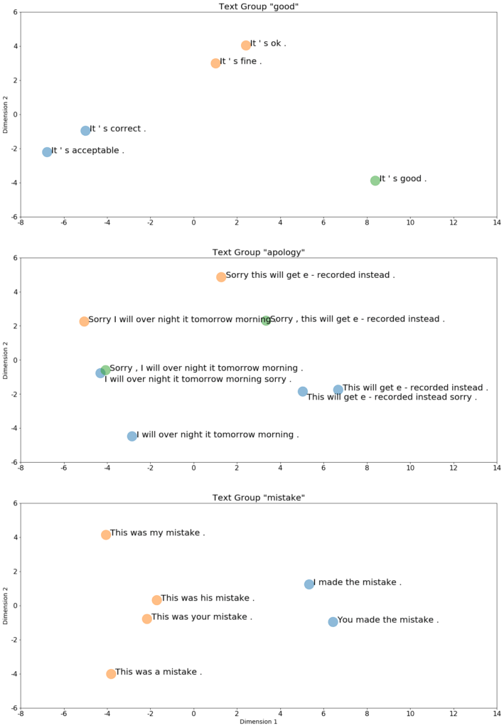
In order to visualize and compare the high dimension vectors of these sentences, we applied principal component analysis (PCA) to reduce them to two dimensions. On the following plots, the x- and y-axes represent the eigenvectors of the 1st and 2nd principal components, respectively. The values are the corresponding eigenvalues.
Figure 1. We colored the data points to show some of the groupings that emerged during this exercise.
Before conducting this experiment, we did not anticipate significant deviations between our example sentences and the representations that the trained model produced. Instead, we saw some fascinating clusters emerge on the PCA plots, and it was an enjoyable process to interpret what the trained model may have seen or learned to produce the patterns.
In the “good” group (Figure 1, first plot), the sentences were all meant to be short affirmations to a request seeking approval, for example “Please let me know if the form looks ok.” After plotting this data, we observed three clusters. “It’s acceptable” and “It’s correct” use more formal language as compared to the rest. Their positions on the plot indicate BERT finds these expressions semantically close. Similarly, “It’s ok” and “It’s fine” are also arguably interchangeable expressions. However, “It’s good” has a larger variety of semantic implications. For example, if we were to ask another question, “Do you like the cake?”, “It’s good” constitutes a reasonable answer, while “It’s correct” is nonsensical. To the same question, “It’s ok” conveys considerably less enthusiasm, and could be construed as the opposite of “It’s good.” Our model has learned these subtle distinctions in usage across a large dataset.
Clustering was more apparent within the “apology” and “good” text groups (Figure 1, second and third plots). In the “apology” group, sentences starting with the word “Sorry” get higher values on the y-axis – especially when “Sorry” was not separated by an additional comma token. In the “mistake” group, sentences with “mistake” playing different syntactic roles clearly map to different representations through the model. Sentences where “mistake” acts as a direct object fall on the left side of the plot. The right side of the plot contains cases where a noun follows a possessive pronoun.
PCA gives us the insight that BERT representations for these sentences differ. Next, we dove into the attention patterns across all layers to visualize BERT’s attention distribution under the hood.
Visualize attention with respect to specific tokens
Let’s first recap what attention scores are. In a BERT model, each word (or token) gets a set of “attention” values (basically an array of numbers) coming from its fellow tokens. The amount of attention “paid by” a token to another can be seen as a measure of importance for the relationship between the two. The model then takes the value of this attention into account to fine-tune the semantic representation. For example, in a task of machine translation, each token in the input sequence gets an attention score; these scores are used to decide which of the input tokens is of importance at a specific point of time in the output sequence, thereby enabling the output of the correct word (in the translated language’s vocabulary). Calculating attention to specific tokens could help us interpret a model’s decisions.
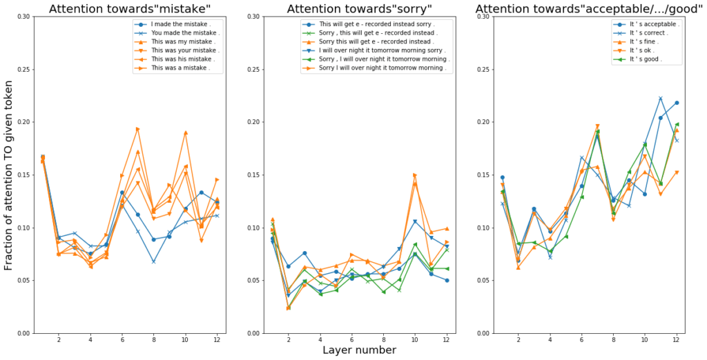
For each group, we select a word that is common or takes the same syntactic role across all examples. We calculated the amount of attention paid to the token from others in the same group (see Appendix for code sample). Note that since the BERT architecture has twelve layers, there are twelve such attention values for each sentence. Plotted against the layer numbers (Figure 2), these attention values towards the chosen tokens show interesting trends. Specifically, for each group, the average attention values were similar in the shallower layers and diverged in the deeper layers as the semantics became more differentiated (semantics disambiguation, as a more complex, higher-level language processing is reported to be a job performed in the latter BERT layers). This observation corresponded with the presence of clusters within the final-layer BERT embeddings (Figure 1).
For the “apology” and “good” groups, a higher amount of attention was paid respectively to a beginning-of-sentence “Sorry” and the words expressing formal approval (“acceptable”, “correct”) (Figure 2, second and third plots). This highlighted that these words were likely key in causing the model’s eventual semantics representations. The “mistake” group is somewhat different, where the word “mistake” clearly took on different syntactic roles. The divergence of attention distribution happened earlier as compared to the “apology” and “good” groups (Figure 2, first plot). This gave us the opportunity to visualize the attention distribution between “mistake” and each token given a specific layer and head using code from Clark et al.’s research. The study associated certain BERT attention heads with specific syntactic relationships. Relevantly, they found that Head 8-10 had direct objects attending to their verbs, and Head 7-6 had possessive pronouns attending to their noun phrases. In our examples, we found multiple heads in Layers 9 and 7 that showed these relationships involving “mistake.”


Conclusions
Visualizing the inner workings of BERT was helpful for understanding how and why sentences that may seem similar can provide interesting challenges to downstream modeling tasks. It’s worth noting that BERT’s behavior is more complex than a general trend in the attention values, and we must be cautious not to leap to too many conclusions with just these simple examples. Nevertheless, the analysis does impart some predictability on the model behavior and give us a level of confidence to implement measures that handle certain language patterns – for instance on short sentences containing emotive expressions.
Feel free to apply these methods on your next BERT model!
Appendix:
How BERT works
Many good introductions have been written about its architecture, which progressively enriches the representation of a sentence over 12 layers. Here’s just a brief recap for what goes on in one such layer (known as a transformer-encoding layer):
- An input text document is tokenized (in BERT’s special way).
- Each token is initialized with an embedding vector.
- Each token’s embedding vector is compared against every other’s via a (scaled) dot product, to calculate a compatibility score. (For more ways to calculate this compatibility score, refer to here).
- The scores are normalized through a softmax.
- The normalized scores are then multiplied back to each of the embedding vectors like a set of weights. The result is then summed to produce a new, composite and nuanced embedding vector for each token.
- Such transformation is repeated 12 times in each layer through a unit called a self-attention head. Subsequent feed-forward, residual connection, and layer normalization mechanisms produce an overall token representation of the encoding layer.
Text examples we used for the analysis
texts_groups = {
"mistake":
   [
       "I made the mistake.",
       "You made the mistake.",
       "This was my mistake.",
       "This was your mistake.",
       "This was his mistake.",
       "This was a mistake."
   ],
"apology":
   [
       "This will get e-recorded instead.",
       "This will get e-recorded instead sorry.",
       "Sorry this will get e-recorded instead.",
       "I will over night it tomorrow morning.",
       "I will over night it tomorrow morning sorry.",
       "Sorry I will over night it tomorrow morning."
   ],
"good":
   [
       "It's acceptable.",
       "It's correct.",
       "It's fine.",
       "It's ok.",
       "It's good.",
   ]
}
Get embeddings and attention scores
First, we start by loading our fine-tuned BERT model — developed using Huggingface’s very useful PyTorch transformer library :
from transformers import BertTokenizer, BertModel, BertForSequenceClassification
tokenizer = BertTokenizer.from_pretrained(MODEL_DIR, do_lower_case=False)
embedder = BertModel.from_pretrained(MODEL_DIR, output_hidden_states=True, output_attentions=True)
By setting output_hidden_states and output_attentions as True, embedder gives the last-layer token embeddings for our sentences, and attention scores in each layer. Using the “mistake” text group as an example, here is sample code:
import torch
import numpy as np
texts = texts_groups['mistake']
# Prepare texts for inference
tokenized_texts = [tokenizer.tokenize(t) for t in texts]
input_ids, masks = get_token_ids(tokenized_texts, 30)
input_ids = torch.tensor(input_ids)
masks = torch.tensor(masks)
# Make an inference and get model outputs
with torch.no_grad():
outputs = embedder(input_ids, masks)
embeddings = outputs[0]
attention_layers = outputs[-1]
# Format the outputs
embeddings = embeddings.numpy().mean(axis=0)
attention_layers = np.array([l.numpy() for l in attention_layers])
Note: get_token_ids() pads and truncates a batch of text-tokens to prepare them as inputs to the BERT model.
We averaged embeddings to create a single embedding for a batch of sentences. In this case, embeddings is shaped like (6, 768) where
- 6 is the number of sentences in our “mistake” text group.
- 768 is the final embedding dimension from the pre-trained BERT architecture.
Attention_layers are converted to a Numpy array. This array has a shape of (12, 12, 30, 30)
- The first dimension is the number of transformer encoder layers, or BERT layers. This value is 12 for the BERT-base-model architecture.
- The second dimension is the number of attention-heads on each layer. This value is (potentially confusingly) also 12 for the BERT-base-model architecture.
- The third and fourth dimensions are the number of tokens, including padding, in each of our sentences. We chose a small value (30) for this analysis. The 30 x 30 attention-score matrix, given a layer and head, represents the amount of attention each token is paying to another, including itself, punctuations, and special BERT tokens such as [CLS] and [SEP].
PCA plots
from sklearn.decomposition import PCA
pca = PCA(n_components=2)
# With tokens, predictions, embeddings from a text group
embeddings_pca = pca.fit_transform(embeddings)
fig, ax = plt.subplots()
For i in range(embeddings_pca.shape[0]):
text = ‘ ‘.join(tokens[i])
pred = predictions[I]
ax.scatter(embeddings_pca[i, 0], embeddings_pca[i, 1], s=500, color='C'+str(pred), alpha=.5)
ax.text(embeddings_pca[i, 0] + 0.2, embeddings_pca[i, 1] - 0.05, text, fontsize=20)
Calculating average attention
The following code computes the average attention towards “mistake” in the sentence “I made the mistake.”
# With tokens, attentions from the sentence
word = “mistake”
token_position = 4
padding_ends = len(tokens) + 2
for num_layer in range(attentions.shape[0]):
for num_head in range(attentions.shape[1]):
attention = attentions[num_layer, num_head, :padding_ends, :padding_ends]
average_attention = attention[:, token_position].sum(-1).mean()